Monte Carlo
Prediction Problem
- An approach that can be used to estimate the state-value function.
- Given a policy, how might the agent estimate the value function for that policy?
Gridworld Example
- The agent has a policy in mind, it follows the policy to collect a lot of episodes.
- For each state, to figure out which action is best, the agent can look for which action tended to result in the most cumulative reward.

Monte Carlo Methods. Image from Udacity nd893
Monte Carlo (MC) Methods
- Even though the underlying problem involves a great degree of randomness, we can infer useful information that we can trust just by collecting a lot of samples.
- The equiprobable random policy is the stochastic policy where - from each state - the agent randomly selects from the set of available actions, and each action is selected with equal probability.
MC prediction (MDP)
- Monte Carlo (MC) approaches to the prediction problem
- The agent can take a bad policy, like the equiprobable random policy, use it to collect some episodes, and then consolidate the results to arrive at a better policy.
- Algorithms that solve the prediction problem determine the value function $v_{\pi}$ or $q_{\pi}$
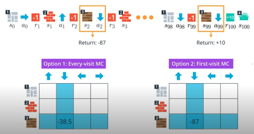
- Each occurrence of the state-action pair $s$, $a$ ($s \in S$, $a \in A$) in an episode is called a visit to $s$, $a$.
Two types of MC prediction
-
Every-visit MC Prediction
- Average the returns following all visits to each state-action pair, in all episodes.
-
First-visit MC Prediction
- For each episode, we only consider the first visit to the state-action pair.
Q-table
- When working with finite MDPs, we can estimate the action-value function $q_{\pi}$ corresponding to a policy $\pi$ in a table.
- This table has one row for each state and one column for each action.
- The entry in the $s$-th row and $a$-th column contains the agent’s estimate for expected return that is likely to follow, if the agent starts in state $s$, selects action $a$, and then henceforth follows the policy $\pi$.
MC Prediction, image from Udacity nd893
First-visit vs Every-visit
- Both the first-visit and every-visit method are guaranteed to converge to the true action-value function, as the number of visits to each state-action pair approaches infinity.
- As long as the agent gets enough experience with each state-action pair, the value function estimate will be pretty close to the true value.
- In the case of first-visit MC, convergence follows from the Law of Large Numbers, and the details are covered in section 5.1 of the textbook.
- Differences
- Every-visit MC is biased, whereas first-visit MC is unbiased (see Theorems 6 and 7).
- Initially, every-visit MC has lower mean squared error (MSE), but as more episodes are collected, first-visit MC attains better MSE (see Corollary 9a and 10a, and Figure 4).
- Ref - Reinforcement Learning with Replacing Eligibility Traces
Greedy Policy
- A greedy policy means the agent constantly performs the action that is believed to yield the highest expected reward.
- With respect to an action-value function estimate $Q$ if for every state $s \in S$, it is guaranteed to select an action $a \in A(s)$ such that $a = argmax_{a \in A_{s}}Q(s,a)$.
- The greedy action: the selected action $a$.

greedy-policy, image from Udacity nd893
Epsilon-Greedy Policy
- Greedy Policy:
- always selects the greedy action
- Epsilon-Greedy Policy:
- most likely selects the greedy action, with probability $1 - \epsilon$
- picks up other non-greedy actions with small, but non-zero probability $\epsilon$
- the agent selects an action uniformly at random from the set of available (non-greedy AND greedy actions)
- allowing the agent to explore other probabilities
- when $\epsilon = 0$, the policy becomes a greedy policy
- when $\epsilon = 1$, the policy becomes an epsilon-greedy policy that is equivalent to the equiprobable random policy
- where, from each state, each action is equally likely to be selected
Control Problem
- Estimates the optimal policy
MC Control Method
- Algorithms designed to solve the control problem determine the optimal policy $\pi_*$ from interaction with the environment.
- The MCC method uses alternating rounds of policy evaluation and improvement to recover the optimal policy.
Two Steps of MC Control
- Policy Evaluation: determine the action-value function of the policy
- Policy Improvement: improve the policy by changing it to be $\epsilon$-greedy with respect to the Q-table

MC Control, image from Udacity nd893
Exploration-Exploitation Dilemma
- In early episodes,
- the agent’s knowledge is quite limited (and potentially flawed).
- So, it is highly likely that actions estimated to be non-greedy by the agent are in fact better than the estimated greedy action.
- With this in mind, a successful RL agent cannot act greedily at every time step (that is, it cannot always exploit its knowledge)
- in order to discover the optimal policy, it has to continue to refine the estimated return for all state-action pairs (in other words, it has to continue to explore the range of possibilities by visiting every state-action pair).
- That said, the agent should always act somewhat greedily, towards its goal of maximizing return as quickly as possible. This motivated the idea of an $\epsilon$-greedy policy.
- Therefore, the agent begins its interaction with the environment by favoring exploration over exploitation. After all, when the agent knows relatively little about the environment’s dynamics, it should distrust its limited knowledge and explore, or try out various strategies for maximizing return.
- At later time steps, it makes sense to favor exploitation over exploration, where the policy gradually becomes more greedy with respect to the action-value function estimate.
- After all, the more the agent interacts with the environment, the more it can trust its estimated action-value function.
Solution: Early Sampling and Late Specialization
One potential solution to this dilemma is implemented by gradually modifying the value of $\epsilonϵ$ when constructing $\epsilon$-greedy policies.
- The best starting policy is the equiprobable random policy, as it is equally likely to explore all possible actions from each state.
- $\epsilon_i >0$ for all time steps $i$
- The later policy becomes more greedy
- $\epsilon_i$ decays to $0$ in the limit as the time step $i$ approaches infinity ($lim_{i \to \infty}\epsilon_i = 0$)
- To ensure convergence to the optimal policy, we could set $ \epsilon_i = \frac 1 i $
Greedy in the limit with Infinite Exploration (GLIE)
- A condition to guarantee that MC control converges to the optimal policy $\pi$
- every state-action pair $s$, $a$ (for all $s \in S$ and $a \in A_{(s)}$) is visited infinitely many times
- the policy converges to a policy that is greedy with respect to the action-value function estimate $Q$
- The condition ensures that
- the agent continues to explore for all time steps
- the agent gradually exploits more (and explore less)
Setting $\epsilon$ in Practice
Even though convergence is not guaranteed by the mathematics, you can often get better results by either:
- using fixed $\epsilon$
- letting $\epsilon_i$ decay to a small positive number, like $0.1$.
- If you get late in training and $\epsilon$ is really small, you pretty much want the agent to have already converged to the optimal policy, as it will take way too long otherwise for it to test out new actions!
- An example of how the value of $\epsilon$ was set in the famous DQN algorithm by reading the Methods section of Human-level control through deep reinforcement learning
The behavior policy during training was epsilon-greedy with epsilon annealed linearly from 1.0 to 0.1 over the first million frames, and fixed at 0.1 thereafter.
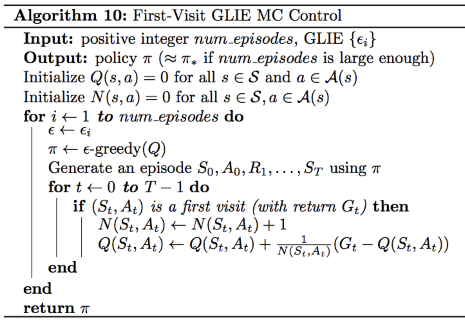
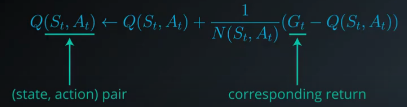
Incremental Mean
- Update the Q-table after every episode.
- Use the updated Q-table to improve the policy.
- That new policy could then be used to generate the next episode, and so on.
- There are two relevant tables
- $Q-Q$ table: with a row for each state and a column for each action . The entry corresponding to state and action is denoted $Q(s,a)$.
- $N$ table: keeps track of the number of first visits we have made to each state-action pair
- The number of episodes the agent collects is equal to $num_episodes$
- The algorithm proceeds by looping over the following steps to improve the policy after every episode
- The policy $\pi$ is improved to be $\epsilon$-greedy with respect to $Q$, and the agent use $\pi$ to collect an episode.
- $N$ is updated to count the total number of first visits to each state action pair
- The estimates in $Q$ are updated to take into account the most recent information
Incremental Mean, image from Udacity nd893
Incremental Mean Function, image from Udacity nd893
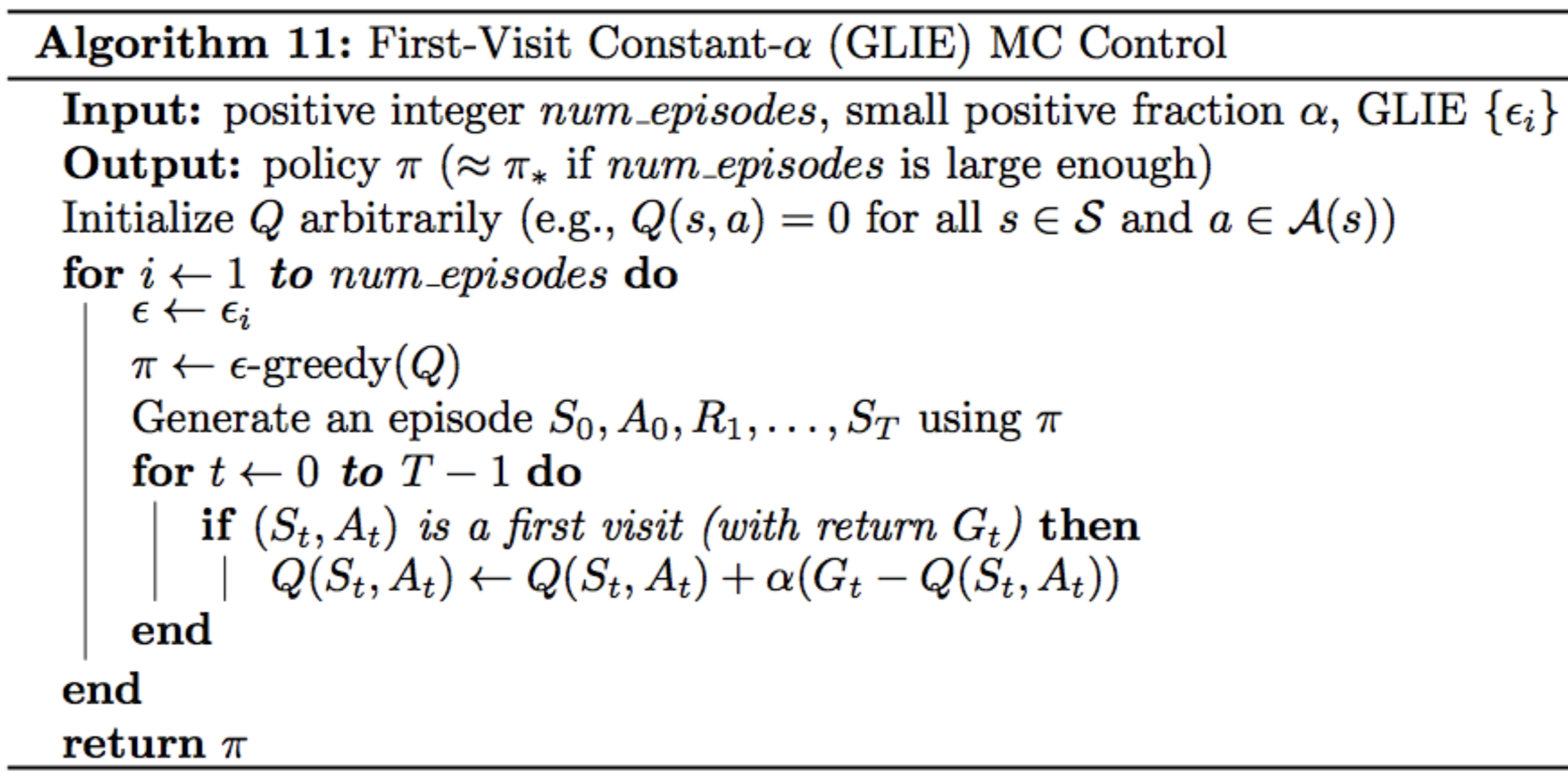
Constant-alpha MC control
- uses a constant step-size parameter $\alpha$
Update equation
-
After each episode finishes, the Q-table is modified using the update equation:
- $Q(S_t, A_t) \leftarrow (1-a)Q(S_t, A_t) + \alpha G_t$
- $G_t := \sum_{s=t+1}^{T}\gamma^{s-t-1}R_s$ is the return at timestep $t$
- $Q(S_t,A_t)$ is the entry in the Q-table corresponding to state $S_t$ and action $A_t$.
-
The main idea behind the update equation
- $Q(S_t,A_t)$ contains the agent’s estimate for the expected return if the environment is in state $S_t$ and the agent selects action $A_t$
- If the return $G_t$ is not equal to $Q(S_t,A_t)$, then we push the value of $Q(S_t,A_t)$ to make it agree slightly more with the return
- The magnitude of the change that we make to $Q(S_t,A_t)$ is controlled by $\alpha > 0$
Step-size Parameter $\alpha$
- The step-size parameter $\alpha$ must satisfy 0 < $\alpha$ ≤1.
- Higher values of $\alpha$ will result in faster learning, but values of $\alpha$ that are too high can prevent MC control from converging to $\pi_*$
- Smaller values for $\alpha$ encourage the agent to consider a longer history of returns when calculating the action-value function estimate.
- Increasing the value of $\alpha$ ensures that the agent focuses more on the most recently sampled returns.
- However,be careful to not set the value of $\alpha$ too close to 1. This is because very large values can keep the algorithm from converging to the optimal policy $\pi_*$
- Boundary values
- If $\alpha = 0$, then the action-value function estimate is never updated by the agent. Meaning, the agent never learns
- If $\alpha = 1$, then the final value estimate for each state-action pair is always equal to the last return that was experienced by the agent (after visiting the pair).
Excercise
OpenAI Gym: BlackJackEnv

Optimal Policy and State-Value Function in Blackjack (Sutton and Barto, 2017)
OpenAI Gym: FrozenLake-v0
- Walking on the ice
- The agent is rewarded for finding a walkable path to a goal tile.
- The solutions are ranked according to the number of episodes needed to find the solution.

Test
Greedy Policy
Which of the values for epsilon yields an epsilon-greedy policy where the agent has the possibility of selecting a greedy action, but might select a non-greedy action instead? In other words, how might you guarantee that the agent selects each of the available (greedy and non-greedy) actions with nonzero probability?
-
- $\epsilon = 0$
-
- $\epsilon = 0.3$
-
- $\epsilon = 0.5$
-
- $\epsilon = 1$
As long as epsilon > 0, the agent has nonzero probability of selecting any of the available actions. So the answer is
2,3,4
Update Q-table
What is the new value for the entry in the Q-table corresponding to state 1 and action right?
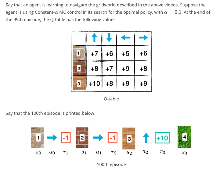
MC Control Method Quiz from Udacity nd893
Answer: 6 + 0.1(8-2) = 6.2 Current estimate: 6 Current reward: 8 $\alpha = 0.1$